pegainfer (3): From Launch Overhead to CUDA Graph (Part 1)
Every time the CPU submits a kernel to the GPU, it goes through a series of driver and runtime calls. This process takes about 4-6 μs. When the kernel’s own computation time is only tens of microseconds, launch overhead can account for 7-10% and create visible gaps on the GPU timeline.
There are roughly four approaches to eliminate this overhead:
| Approach | Core Idea | Implementation Difficulty | Limitations |
|---|---|---|---|
| CUDA Graph | Record once, replay many times | Low | Parameters frozen, harder to debug |
| Kernel Fusion | Merge multiple kernels into one | Medium | Fusion complexity, register pressure |
| Mega Kernel | Ultimate fusion, only one kernel left | High | Poor maintainability, needs compiler assistance |
| Dynamic Parallelism | GPU launches kernels itself | Low | Limited performance gain, not observable |
This post first quantifies how large launch overhead actually is, then experiments with all four approaches and compares them. CUDA Graph, being the most commonly used approach, will be covered in detail; the others serve as comparisons. The next post will cover how to integrate CUDA Graph into a real inference framework and related profiling practices.
Experiment environment: NVIDIA GeForce RTX 5070 Ti (16 GB), Driver 580.126.09, CUDA 13.0 Code: https://github.com/xiaguan/cuda-kernel-launch-lab
Start with a simple GPU kernel that consumes some GPU time.
__global__ void shortKernel(float *data) {
  int idx = blockIdx.x * blockDim.x + threadIdx.x;
  if (idx < N) {
    float v = data[idx];
    #pragma unroll
    for (int i = 0; i < 20; i++) v = sinf(v) * 0.99f + 0.01f;
    data[idx] = v;
  }
}
We call this kernel frequently and wait for it to finish each time.
  for (int istep = 0; istep < NSTEP; istep++) {
    for (int ikrnl = 0; ikrnl < NKERNEL; ikrnl++) {
      shortKernel<<<blocks, THREADS, 0, stream>>>(out_d);
      CHECK(cudaStreamSynchronize(stream));
    }
  }
We measure the total time of the two for loops, which includes both kernel launch and kernel computation time.
But what we want to know is the kernel launch time. Just subtract the kernel computation time from the total. Pure computation time can be obtained by submitting multiple kernels consecutively (without inserting sync) and timing with CUDA Events. Note that this requires the kernel computation time to be greater than the launch time, otherwise kernels will queue up waiting for the previous one to finish, and what you measure won’t be pure computation time.
  cudaEvent_t ev_start, ev_stop;
  CHECK(cudaEventCreate(&ev_start));
  CHECK(cudaEventCreate(&ev_stop));

  const int NRUNS = 100;
  CHECK(cudaEventRecord(ev_start, stream));
  for (int i = 0; i < NRUNS; i++) {
    shortKernel<<<blocks, THREADS, 0, stream>>>(out_d);
  }
  CHECK(cudaEventRecord(ev_stop, stream));
  CHECK(cudaEventSynchronize(ev_stop));

  float kernel_ms = 0;
  CHECK(cudaEventElapsedTime(&kernel_ms, ev_start, ev_stop));
The measured result shows kernel launch overhead is around 5.7us.
Kernel execution time (CUDA event):  47.16 us
Naive per-kernel time (wall clock):  52.92 us
Overhead per kernel:                 5.75 us  (12%)
But this is just inferred from external timing. We can use NVIDIA’s profiling tool nsys to confirm the kernel launch time.
nsys profile -o naive_report --export sqlite ./naiveThis generates two files:
naive_report.nsys-rep (nsys native format, NVIDIA has a UI to view it)
naive_report.sqlite  (sqlite format)
Since I’m SSHing into the machine and don’t have a GPU machine with a UI at hand, we use the sqlite format with an open-source script (https://github.com/chenyu-jiang/nsys2json, converts to chrome tracing json, scp to Mac, then view in the Mac browser).
 Look at the overall timing.
 Kernel launch takes about 4.1us, close to our estimate. Kernel computation time is about 47us. From kernel completion to stream sync return, there’s also a 1us+ gap. At the same time, the GPU stream below has visible gaps, causing GPU idle time.
So we originally only needed 47us of computation time, but now we’re spending an extra 4us, roughly 9% more. When kernel computation time is shorter, this problem becomes more obvious.
How to eliminate this overhead? We listed four approaches at the beginning. Let’s experiment with them one by one. Starting with CUDA Graph.
(Side note: kernel launch is like a traditional CPU syscall. How does io_uring eliminate the submission syscall? The kernel spawns a thread to poll.)
For CUDA Graph, you can refer to NVIDIA’s own resources:
- https://developer.nvidia.com/blog/cuda-graphs/ CUDA Graph introduction
- https://docs.nvidia.com/cuda/cuda-programming-guide/04-special-topics/cuda-graphs.html , CUDA Graph official documentation
CUDA Graphs present another model for work submission in CUDA. This allows a graph to be defined once and then launched repeatedly.
CUDA Graphs is another form of submission. It’s defined once, then replayed many times. We create a CUDA Graph to encapsulate a workflow that will be launched many times, record it, and then just replay this graph. Replay only needs to submit one Graph, with minimal overhead.
For its definition, usage, API, and details, please refer to the official documentation. We capture the inner loop of the previous double for loop (20 kernel launches).
  // ---- Graph capture: capture the inner NKERNEL launches ----
  cudaGraph_t graph;
  cudaGraphExec_t graphExec;

  CHECK(cudaStreamBeginCapture(stream, cudaStreamCaptureModeGlobal));
  for (int i = 0; i < NKERNEL; i++) {
    shortKernel<<<blocks, THREADS, 0, stream>>>(out_d);
  }
  CHECK(cudaStreamEndCapture(stream, &graph));
CHECK(cudaGraphInstantiate(&graphExec, graph));cudaGraph_tis the result of recordingcudaGraphExec_tis the object that can be used for replay later
cudaStreamBeginCapture(stream, cudaStreamCaptureModeGlobal)Start recording operations on the specified stream, but don’t execute them, just record. cudaStreamCaptureModeGlobal is the strictest mode, preventing other streams from interfering during recording. Other modes are also available.
Then we submit kernels. The GPU is recording, silently building a graph:
Node1(shortKernel(args)) -> Node2(shortKernel(args)) -> Node20Then call cudaStreamEndCapture to end recording, pack it into a cudaGraph_t and return. The stream goes back to normal mode.
cudaGraph_t can’t be used for replay yet. We still need to instantiate it and check if the graph’s internal structure is valid, by calling:
cudaGraphInstantiate(&graphExec, graph)If no error is returned, cudaGraphExec_t is the graph object we can use for replay. After that, replay is very simple:
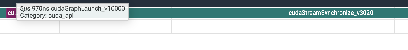
  for (int istep = 0; istep < NSTEP; istep++) {
    CHECK(cudaGraphLaunch(graphExec, stream));
    CHECK(cudaStreamSynchronize(stream));
  }
Let’s directly compare performance:
Naive per-kernel time (wall clock):  52.92 us (non-graph)
Graph per-kernel time (wall clock):  46.98 us (graph version)
Each kernel is nearly 6us faster, as expected. Let’s see what the nsys trace looks like.
 Why is the GPU stream empty? Turns out we need to add a flag
 --cuda-graph-trace=node to nsys. After rerunning:
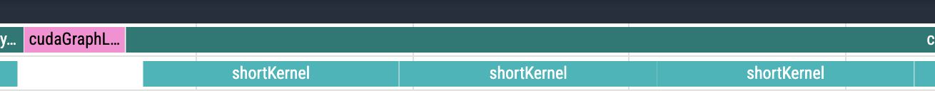 After one graph launch, the CPU side enters waiting, while the GPU side processes kernels very tightly, with almost no gaps.
In this scenario it looks simple. Is it really this easy? Let’s look at Graph’s drawbacks:
- Recording and instantiation have overhead
- Parameters are fixed, the graph is frozen
Which kernels are called, the order, all parameters — everything is frozen. When calling
cudaGraphLaunch, there’s no room to pass parameters. But parameters are usually pointers. The pointer itself is frozen, but the data at the address the pointer points to can change. - Harder to debug. After graph launch, there are no CPU operations — no print, no logging — making debugging harder.
- Not all operations can be recorded. Basically only pure GPU operations can be recorded. Anything that might involve CPU intervention probably can’t, like
cudaMalloc. - Graphs consume GPU memory. The instantiated graph is stored on the GPU, and its size is proportional to graph complexity.
Next let’s look at kernel fusion. Literally, it means writing multiple kernels as one kernel. Here’s a visual example: https://www.abhik.ai/articles/kernel-fusion. For instance, the inner for loop calling a small kernel 20 times can be written as one kernel with an internal loop, so you only need to launch once.
// Fused kernel: one launch completes NKERNEL steps
__global__ void fusedKernel(float *data) {
  int idx = blockIdx.x * blockDim.x + threadIdx.x;
  if (idx < N) {
    float v = data[idx];
    for (int k = 0; k < NKERNEL; k++) {
      #pragma unroll
      for (int i = 0; i < 20; i++) v = sinf(v) * 0.99f + 0.01f;
    }
    data[idx] = v;
  }
}
Decent performance improvement:
Fusion per-kernel time (wall clock): 44.43 usThe improvement comes from two aspects: first, eliminating 19 kernel launch overheads; second, after fusion, intermediate results stay in registers the whole time, saving 19 global memory reads/writes (~8MB each), reducing a lot of memory bandwidth consumption. The latter belongs to operator optimization, which we won’t expand on here.
Benefits of kernel fusion:
- Eliminates kernel launch
- Reduces intermediate result memory reads/writes, data stays in registers/shared memory
- Possible additional performance gains (instruction-level parallelism, etc.)
Drawbacks:
- Not all kernels are as easy to fuse as the one above. Fusion increases complexity and reduces maintainability.
- Register pressure and other detailed operator issues — we’ll expand on these later.
Generally, do fusion first, then try Graph. The two don’t conflict.
So what is MegaKernel (also called persistent kernel)? It’s the ultimate fusion — fusing until only one kernel remains. From all kinds of computation to inter-GPU communication, just one kernel! In this post’s example, it means wrapping the outer loop in too:
// mega kernel: NSTEP × NKERNEL × 20 sinf all done
__global__ void megaKernel(float *data) {
  int idx = blockIdx.x * blockDim.x + threadIdx.x;
  if (idx < N) {
    float v = data[idx];
    for (int step = 0; step < NSTEP; step++) {
      for (int k = 0; k < NKERNEL; k++) {
        #pragma unroll
        for (int i = 0; i < 20; i++) v = sinf(v) * 0.99f + 0.01f;
      }
    }
    data[idx] = v;
  }
}
Still some improvement:
Mega per-kernel time (wall clock): 43.92 usIn this example, we intentionally wrote such a simple kernel to help readers understand. But in the real world, I recommend reading last year’s Stanford Megakernel paper on Llama-1B (https://hazyresearch.stanford.edu/blog/2025-05-27-no-bubbles, it also optimizes for bs=1, where computation is small, kernels are fast, and launch overhead proportion is large, sponsored by Together). They needed to fuse about a hundred operators. They didn’t write them by hand either — they built a compiler-like thing to generate them.
Finally, Dynamic Parallelism, or CDP for short. The core idea in one sentence: let the GPU launch kernels instead of the CPU.
It’s also fairly simple to write — it really is just calling kernels inside kernels:
// parent kernel: single-thread scheduler, launches NKERNEL child kernels on GPU
__global__ void parentKernel(float *data, int blocks) {
  // CDP2: child grids implicitly synchronize before parent thread block exits
  for (int k = 0; k < NKERNEL; k++) {
    shortKernel<<<blocks, THREADS>>>(data);
  }
}
Two extra compilation options are needed:
-rdc=true, Relocatable Device Code. In normal compilation, device code is “self-contained” and can’t call across compilation units. With rdc enabled, device code can call other device functions — DP needs this because the parent kernel needs to “see” the child kernel’s symbol to launch it.-lcudadevrt, links the CUDA device runtime library, providing the GPU-side kernel launch mechanism.
Performance is slightly better than the naive version, but worse than Graph.
Let’s look at its profile trace. We still need to launch one parent kernel. What about the child kernels?
 After Opus 4.6 spent a while struggling with the sqlite, it said nsys currently can’t profile CDP2’s child kernels. This is also one of its drawbacks — not observable.
The above are all toy kernels. But in a real inference framework, each decode step runs dozens of different kernels, with parameters changing and shapes changing. How do you integrate Graph? Is it complicated? How much faster does it get?
The next post will discuss the process of actually integrating CUDA Graph into pegainfer, what pitfalls were encountered, and how much faster decode actually got.